STAVER shows robust generalization across various large-scale DIA datasets¶

To further validate the reliability of STAVER’s results and underscore the robustness and inherent advantages of the STAVER algorithm, we applied STAVER to a much more diverse and larger-scale DIA dataset from the “ProCan-DepMap-Sanger project” (Gonçalves, et al. 2022, Cancer Cell). A total of 1,326 samples were included for analysis, including 84 samples of HEK293T cell lines used for quality control and 1,242 cancer cell samples derived from 9 typical cancer types (colorectal, SCLC, kidney, gastric, pancreatic, bladder, NSCLC, glioma, and hepatocellular cancer) (Figure RL2A-RL2B and Figure RL5A-RL5B).

We performed a comprehensive comparative analysis of the original data without the STAVER processing and the STAVER-processed data, with the main results focusing on - (I) the reproducibility and reliability of the STAVER-processed data, - (II) the robustness of the STAVER algorithm to uncover inherent biological differences, - (III) the reproducibility of the STAVER algorithm in identifying the previously reported tumor biomarkers, and - (IV) the robustness and broad applicability of the STAVER algorithm for disease diagnosis and classification.

[1]:

import pandas as pd
import numpy as np
import plotly.express as px
import plotly.io as pio
import plotly.graph_objects as go
import colorsys
import seaborn as sns
import matplotlib as mpl
import matplotlib.pyplot as plt
import scanpy as sc
import anndata
import os
import matplotlib.pyplot as plt
# python matplotlib export editable PDF
import matplotlib as mpl
mpl.rcParams['pdf.fonttype'] = 42
# mpl.rcParams['figure.dpi']= 150

import warnings
warnings.filterwarnings('ignore')

from plotly.offline import init_notebook_mode, iplot
init_notebook_mode(connected=True)

Metadata¶

[2]:

metadata = pd.read_excel("~/STAVER-revised/Pan-cancer-cell-lines/subset_949_samples.xlsx",index_col=0)
metadata

[2]:

	Automatic_MS_filename	Batch	Date	Instrument	Cell_line	SIDM	Tissue_type	Cancer_type	Cancer_subtype	Project_Identifier
519	191012_b36-t2-8_00di6_00jm7_m06_s_1	P04	2019-10-12	M06	BFTC-905	SIDM00989	Bladder	Bladder Carcinoma	Urothelial carcinoma	SIDM00989;BFTC-905
521	191023_b61-t1-1_00dsu_00kp3_m03_s_1	P04	2019-10-23	M03	BFTC-905	SIDM00989	Bladder	Bladder Carcinoma	Urothelial carcinoma	SIDM00989;BFTC-905
522	191026_b36-t3-8_00di6_00kt6_m04_s_1	P04	2019-10-26	M04	BFTC-905	SIDM00989	Bladder	Bladder Carcinoma	Urothelial carcinoma	SIDM00989;BFTC-905
523	191026_b61-t2-1_00dsu_00ktw_m06_s_1	P04	2019-10-26	M06	BFTC-905	SIDM00989	Bladder	Bladder Carcinoma	Urothelial carcinoma	SIDM00989;BFTC-905
524	191125_b32-t4-8_00dge_00n1d_m03_s_1	P04	2019-11-25	M03	BFTC-905	SIDM00989	Bladder	Bladder Carcinoma	Urothelial carcinoma	SIDM00989;BFTC-905
...	...	...	...	...	...	...	...	...	...	...
6590	200131_b4-7-t3-1_00q3n_00rtc_m05_s_1	P06	2020-01-31	M05	COR-L95	SIDM00521	Lung	Small Cell Lung Carcinoma	Small cell lung carcinoma	SIDM00521;COR-L95
6591	200131_b4-9-t3-1_00q3p_00rte_m05_s_1	P06	2020-01-31	M05	NCI-H510A	SIDM00927	Lung	Small Cell Lung Carcinoma	Small cell lung carcinoma	SIDM00927;NCI-H510A
6592	200131_b4-10-t3-1_00q3q_00rtf_m05_s_1	P06	2020-01-31	M05	NCI-H2171	SIDM00733	Lung	Small Cell Lung Carcinoma	Small cell lung carcinoma	SIDM00733;NCI-H2171
6593	200131_b4-13-t3-1_00q3t_00rti_m05_s_1	P06	2020-01-31	M05	NCI-H1836	SIDM00770	Lung	Small Cell Lung Carcinoma	Small cell lung carcinoma	SIDM00770;NCI-H1836
6594	200201_b3-13-t3-2_00q3d_00rtm_m05_s_1	P06	2020-02-01	M05	IST-SL1	SIDM00223	Lung	Small Cell Lung Carcinoma	Small cell lung carcinoma	SIDM00223;IST-SL1

1242 rows × 10 columns

Tissue_type¶

[3]:

Tissue_type_counts = metadata['Tissue_type'].value_counts().reset_index()
Tissue_type_counts.columns = ['Tissue_type', 'Count']
Tissue_type_counts

[3]:

	Tissue_type	Count
0	Lung	273
1	Large Intestine	271
2	Kidney	181
3	Stomach	153
4	Pancreas	115
5	Bladder	96
6	Central Nervous System	78
7	Liver	75

[4]:

fig = px.pie(Tissue_type_counts, values='Count', names='Tissue_type', title="Diverse Tissue Type")
fig.update_traces(textinfo='label+percent', insidetextorientation='radial')

# Save figure to PDF
pio.write_image(fig, 'figs/Tissue_type.pdf')

Cancer_type¶

[5]:

Cancer_type_counts = metadata['Cancer_type'].value_counts().reset_index()
Cancer_type_counts.columns = ['Cancer_type', 'Count']
Cancer_type_counts

[5]:

	Cancer_type	Count
0	Colorectal Carcinoma	271
1	Small Cell Lung Carcinoma	187
2	Kidney Carcinoma	181
3	Gastric Carcinoma	153
4	Pancreatic Carcinoma	110
5	Bladder Carcinoma	96
6	Non-Small Cell Lung Carcinoma	86
7	Glioma	78
8	Hepatocellular Carcinoma	75
9	Other Solid Carcinomas	5

[6]:

fig = px.pie(Cancer_type_counts, values='Count', names='Cancer_type', title="Diverse Cancer Type")
# Update the labels to show both count and percentage
fig.update_traces(textinfo='label+percent', insidetextorientation='radial')

# Save figure to PDF
pio.write_image(fig, 'figs/Cancer_types.pdf')

Cancer_subtype¶

[7]:

Cancer_subtype = metadata['Cancer_subtype'].value_counts().reset_index()
Cancer_subtype.columns = ['Cancer_subtype', 'Count']

Cancer_subtype["Cancer_subtype_modify"] = [
    x if count > 14 else "Others"
    for x, count in zip(Cancer_subtype["Cancer_subtype"], Cancer_subtype["Count"])
]

Cancer_subtype

[7]:

	Cancer_subtype	Count	Cancer_subtype_modify
0	Small cell lung carcinoma	187	Small cell lung carcinoma
1	Colon adenocarcinoma	147	Colon adenocarcinoma
2	Kidney carcinoma	107	Kidney carcinoma
3	Bladder carcinoma	89	Bladder carcinoma
4	Squamous cell lung carcinoma	86	Squamous cell lung carcinoma
5	Gastric adenocarcinoma	75	Gastric adenocarcinoma
6	Hepatocellular carcinoma	72	Hepatocellular carcinoma
7	Low grade glioma	72	Low grade glioma
8	Clear cell renal cell carcinoma	64	Clear cell renal cell carcinoma
9	Pancreatic ductal adenocarcinoma	52	Pancreatic ductal adenocarcinoma
10	Cecum adenocarcinoma	46	Cecum adenocarcinoma
11	Pancreatic adenocarcinoma	44	Pancreatic adenocarcinoma
12	Colorectal carcinoma	43	Colorectal carcinoma
13	Rectal adenocarcinoma	35	Rectal adenocarcinoma
14	Gastric signet ring cell adenocarcinoma	29	Gastric signet ring cell adenocarcinoma
15	Gastric tubular adenocarcinoma	15	Gastric tubular adenocarcinoma
16	Pancreatic carcinoma	13	Others
17	Gastric carcinoma	12	Others
18	Urothelial carcinoma	7	Others
19	Gastric fundus carcinoma	7	Others
20	Papillary renal cell carcinoma	6	Others
21	Oligodendroglioma	6	Others
22	Gastic small cell neuroendocrine carcinoma	6	Others
23	Gastric small cell carcinoma	6	Others
24	Pancreatic somatostatinoma	5	Others
25	Renal pelvis and ureter urothelial carcinoma	4	Others
26	Hepatoblastoma	3	Others
27	Gastric choriocarcinoma	3	Others
28	Pancreatic adenosquamous carcinoma	1	Others

[8]:

fig = px.pie(Cancer_subtype, values='Count', names='Cancer_subtype_modify', title="Diverse Cancer subtype")
# Update the labels to show both count and percentage
fig.update_traces(textinfo='label+percent', insidetextorientation='radial')

# Save figure to PDF
pio.write_image(fig, 'figs/Diverse Cancer subtype modify.pdf')

The Sankey diagram delineates the relationships¶

[9]:

def aggregate_by_sum(df, column_name, threshold=14):

    # Group by the specified column and calculate the sum for each group
    group_counts = df.groupby(column_name).size()

    # Select groups with a sum greater than the threshold
    processed_data = group_counts[group_counts > threshold].index.tolist()

    # Filter the original DataFrame for rows belonging to the filtered groups
    processed_data = df[df[column_name].isin(processed_data)]

    return processed_data

# 使用函数
result_df = aggregate_by_sum(metadata, 'Cancer_subtype', 10)
result_df

[9]:

	Automatic_MS_filename	Batch	Date	Instrument	Cell_line	SIDM	Tissue_type	Cancer_type	Cancer_subtype	Project_Identifier
527	181010_e0022_p02_2178_1_s_m04_1	P02	2018-10-10	M04	SW1710	SIDM00420	Bladder	Bladder Carcinoma	Bladder carcinoma	SIDM00420;SW1710
528	181010_e0022_p02_2178_3_s_m04_1	P02	2018-10-10	M04	SW1710	SIDM00420	Bladder	Bladder Carcinoma	Bladder carcinoma	SIDM00420;SW1710
529	181010_e0022_p02_2178_2_s_m04_1	P02	2018-10-10	M04	SW1710	SIDM00420	Bladder	Bladder Carcinoma	Bladder carcinoma	SIDM00420;SW1710
530	181127_e0022_p02_2051_3_s_m04_1	P02	2018-11-27	M04	RT-112	SIDM00402	Bladder	Bladder Carcinoma	Bladder carcinoma	SIDM00402;RT-112
531	181127_e0022_p02_2051_1_s_m04_1	P02	2018-11-27	M04	RT-112	SIDM00402	Bladder	Bladder Carcinoma	Bladder carcinoma	SIDM00402;RT-112
...	...	...	...	...	...	...	...	...	...	...
6590	200131_b4-7-t3-1_00q3n_00rtc_m05_s_1	P06	2020-01-31	M05	COR-L95	SIDM00521	Lung	Small Cell Lung Carcinoma	Small cell lung carcinoma	SIDM00521;COR-L95
6591	200131_b4-9-t3-1_00q3p_00rte_m05_s_1	P06	2020-01-31	M05	NCI-H510A	SIDM00927	Lung	Small Cell Lung Carcinoma	Small cell lung carcinoma	SIDM00927;NCI-H510A
6592	200131_b4-10-t3-1_00q3q_00rtf_m05_s_1	P06	2020-01-31	M05	NCI-H2171	SIDM00733	Lung	Small Cell Lung Carcinoma	Small cell lung carcinoma	SIDM00733;NCI-H2171
6593	200131_b4-13-t3-1_00q3t_00rti_m05_s_1	P06	2020-01-31	M05	NCI-H1836	SIDM00770	Lung	Small Cell Lung Carcinoma	Small cell lung carcinoma	SIDM00770;NCI-H1836
6594	200201_b3-13-t3-2_00q3d_00rtm_m05_s_1	P06	2020-02-01	M05	IST-SL1	SIDM00223	Lung	Small Cell Lung Carcinoma	Small cell lung carcinoma	SIDM00223;IST-SL1

1188 rows × 10 columns

[10]:

def generate_color_map(labels, alpha_nodes=1.0, alpha_links=0.55):
    hues = [i/len(labels) for i in range(len(labels))]
    colors_hsv = [(h, 0.5, 0.8) for h in hues]

    colors_rgba_nodes = [colorsys.hsv_to_rgb(*hsv) for hsv in colors_hsv]
    colors_rgba_links = [(r, g, b, alpha_links) for r, g, b in colors_rgba_nodes]
    colors_rgba_nodes = [(r, g, b, alpha_nodes) for r, g, b in colors_rgba_nodes]

    colors_str_nodes = ["rgba({},{},{},{})".format(int(r*255), int(g*255), int(b*255), a) for r, g, b, a in colors_rgba_nodes]
    colors_str_links = ["rgba({},{},{},{})".format(int(r*255), int(g*255), int(b*255), a) for r, g, b, a in colors_rgba_links]

    return dict(zip(labels, colors_str_nodes)), dict(zip(labels, colors_str_links))


def draw_sankey(data, filename=None):
    all_labels = sorted(list(set(data['Tissue_type'].unique().tolist() + data['Cancer_type'].unique().tolist() + data['Cancer_subtype'].unique().tolist())))

    node_color_map, link_color_map = generate_color_map(all_labels)

    # Aggregate data
    links = data.groupby(['Tissue_type', 'Cancer_type', 'Cancer_subtype']).size().reset_index(name='count')

    final_source = []
    final_target = []
    final_value = []

    for index, row in links.iterrows():
        final_source.append(all_labels.index(row['Tissue_type']))
        final_target.append(all_labels.index(row['Cancer_type']))
        final_value.append(row['count'])

        final_source.append(all_labels.index(row['Cancer_type']))
        final_target.append(all_labels.index(row['Cancer_subtype']))
        final_value.append(row['count'])

    link_colors = [link_color_map[all_labels[s]] for s in final_source]

    fig = go.Figure(go.Sankey(
        node=dict(
                pad=15,
                thickness=20,
                line=dict(color="black", width=0.5),
                label=all_labels,
                color=[node_color_map[label] for label in all_labels]
        ),
        link=dict(
                source=final_source,
                target=final_target,
                value=final_value,
                color=link_colors
            )
    ))

    fig.update_layout(title_text="Sankey Diagram of Cancer Types and Subtypes", font_size=10)

    if filename:
        fig.write_image(filename)

    fig.show()

# 使用示例
# df = pd.DataFrame(data)
draw_sankey(result_df, filename="sankey_diagram-3.pdf")

The reproducibility and reliability of the STAVER-processed data¶

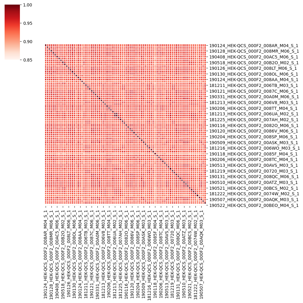
HEK293T Spearman correlation analysis¶

[6]:

# Load HEK293T data
HEK293T_rawdata = pd.read_csv("~/STAVER-revised/HEK_293T/HEK-QCS_matrix_rawdata.csv", index_col=0)
HEK293T_rawdata.dropna(thresh=5, inplace=True)
HEK293T_STAVER = pd.read_csv("~/STAVER-revised/HEK_293T/HEK-QCS_matrix_STAVER.csv", index_col=0)
HEK293T_STAVER.dropna(thresh=5, inplace=True)

[26]:

def correlation_heatmap(data, method = 'pearson', log_transformed = False, outpath = None, filename = None):
    """ Correaltion heatmap and correlation matrix
    Args:
    --------------
    data -> Dataframe: dataframe of raw data
    method -> str: pearson or spearman
    log_transformed -> bool: whether to use log10 transformed data

    Return:
    -----------
    Dataframe: Correaltion of experiments data

    """
    if log_transformed:
        data = np.log10(data)
    corr = data.corr(method = method)
    ## Platelet selection refernce: https://learnku.com/articles/39890
    plt.figure(figsize=(10, 10))
    # optional cmap: RdYlGn; RdYlGn_r; YlGn; rocket_r; YlGnBu; YlGnBu_r; YlOrBr; YlOrBr_r; YlOrRd; YlOrRd_r; RdBu_r
    sns.clustermap(corr, cmap="Reds", annot= False, robust=False, col_cluster=False, row_cluster=False, linewidths=.005,fmt=".2f")
    # sn.heatmap(corr, annot=True, cmap='vlag')  ## optional cmap: RdYlGn; RdYlGn_r; YlGn; rocket_r; YlGnBu; YlGnBu_r; YlOrBr; YlOrBr_r; YlOrRd; YlOrRd_r;
    if outpath:
        plt.savefig(f"{outpath}/{filename}_corr_heatmap.pdf")
        corr.to_csv(f"{outpath}/{filename}_corr_matrix.csv")
    plt.show()
    # return corr

The correlation heatmap of raw data¶

[27]:

outpath = r'~/STAVER-revised/figs/'
correlation_heatmap(HEK293T_rawdata, method = 'spearman', log_transformed=False, outpath = outpath, filename = 'HEK-QCS_matrix_rawdata_corr_heatmap')

<Figure size 1000x1000 with 0 Axes>

_images/PanCancer_949_celline_analysis_21_1.png

The correlation heatmap of STAVER-processed data¶

[28]:

outpath = r'~/STAVER-revised/figs/'
correlation_heatmap(HEK293T_STAVER, method = 'spearman', log_transformed=False, outpath = outpath, filename = 'HEK-QCS_matrix_STAVER_corr_heatmap')

<Figure size 1000x1000 with 0 Axes>

_images/PanCancer_949_celline_analysis_23_1.png

[93]:

def extract_lower_triangular(df_corr):
    """
    提取相关性矩阵对角线以下的一半相关性值。

    参数:
    ----
    df_corr : pandas.DataFrame
        相关性矩阵的 DataFrame。

    返回:
    -----
    pandas.DataFrame
        包含对角线以下一半相关性值的 DataFrame。
    """
    if not isinstance(df_corr, pd.DataFrame):
        raise ValueError("df_corr 必须是 pandas.DataFrame 类型。")

    # 获取对角线以下的索引
    tril_indices = np.tril_indices(df_corr.shape[0], k=-1)

    # 提取对角线以下的一半相关性值
    lower_triangular_values = df_corr.to_numpy()[tril_indices]

    return pd.DataFrame(
        {
            'Row': df_corr.index[tril_indices[0]],
            'Column': df_corr.columns[tril_indices[1]],
            'Correlation': lower_triangular_values,
        }
    )


def get_IQR(data):
    Q1 = data.quantile(0.25)
    Q3 = data.quantile(0.75)
    IQR = Q3 - Q1
    print(f"The IQR1 is: {Q1}")
    print(f"The IQR3 is: {Q3}")
    mean = data.mean()
    print(f"The mean is: {mean}")
    median = data.median()
    print(f"The median is: {median}")

The IQR of HEK293T spearman correlation matrix in rawdata¶

[105]:

res = extract_lower_triangular(HEK293T_rawdata.corr())
get_IQR(res['Correlation'])

The IQR1 is: 0.8846399725
The IQR3 is: 0.907049235
The mean is: 0.893689345854834
The median is: 0.897238564

The IQR of HEK293T spearman correlation matrix in SATVER-processed data¶

[106]:

res = extract_lower_triangular(HEK293T_STAVER.corr())
get_IQR(res['Correlation'])

The IQR1 is: 0.9321159908757065
The IQR3 is: 0.9821799248475355
The mean is: 0.9523831119684066
The median is: 0.9657469442578246

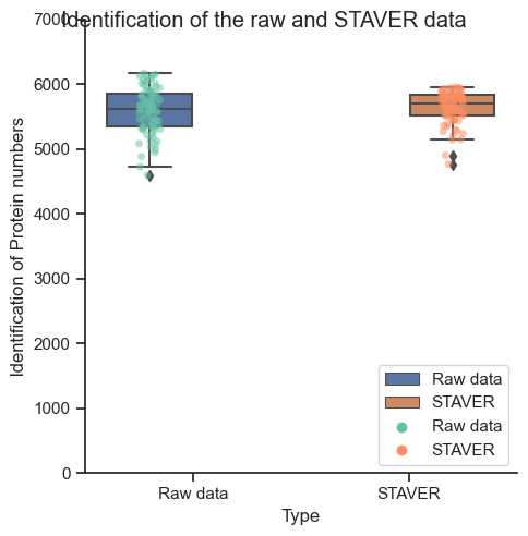
The identification protein numbers of the raw data and STAVER data¶

[2]:

protein_num= pd.read_clipboard()
protein_num

[2]:

	Experiment	ldentification of Protein numbers	Type
0	190124_HEK-QCS_000F2_008AR_M04_S_1	5683	Raw data
1	190124_HEK-QCS_000F2_008IQ_M06_S_1	5923	Raw data
2	190125_HEK-QCS_000F2_008JO_M04_S_1	5617	Raw data
3	190128_HEK-QCS_000F2_008MR_M06_S_1	5873	Raw data
4	190129_HEK-QCS_000F2_008NM_M04_S_1	5465	Raw data
...	...	...	...
162	190102_HEK-QCS_000F2_007K6_M02_S_1	5150	STAVER
163	190401_HEK-QCS_000F2_00A13_M06_S_1	5817	STAVER
164	190507_HEK-QCS_000F2_00AQK_M03_S_1	5961	STAVER
165	190522_HEK-QCS_000F2_00BEO_M04_S_1	5283	STAVER
166	181213_HEK-QCS_000F2_006UR_M03_S_1	5519	STAVER

167 rows × 3 columns

[28]:

def plot_protein_numbers(data, x_col, y_col, title, y_lim=None, height=6, aspect=1.3):
    """
    Creates a combined box and strip plot for protein number visualization.

    Args:
        data (pd.DataFrame): DataFrame containing the data to be plotted.
        x_col (str): Column name in `data` to be plotted on the x-axis.
        y_col (str): Column name in `data` to be plotted on the y-axis.
        title (str): Title of the plot.
        y_lim (tuple, optional): Tuple specifying the limits for the y-axis (e.g., (0, 7000)).
        height (float, optional): Height (in inches) of each facet. Defaults to 6.
        aspect (float, optional): Aspect ratio of each facet, so that aspect * height gives the width of each facet in inches. Defaults to 1.3.

    Example:
        >>> plot_protein_numbers(protein_num, 'Type', 'Identification of Protein numbers',
                                'Protein numbers of HEK293T QC samples', y_lim=(0, 7000), height=5, aspect=1)
    """
    custom_params = {"axes.spines.right": False, "axes.spines.top": False}
    sns.set_theme(style="ticks", rc=custom_params)

    # Create a box plot
    box_plot = sns.catplot(x=x_col, y=y_col, hue=x_col, kind="box", legend=False, height=height, aspect=aspect, data=data)

    # Overlay with a strip plot
    sns.stripplot(x=x_col, y=y_col, hue=x_col, jitter=True, dodge=True, marker='o', palette="Set2", alpha=0.5, data=data)

    # Set additional plot attributes
    box_plot.fig.suptitle(title)  # Set the title for the figure
    plt.legend(loc='lower right')
    if y_lim:
        plt.ylim(y_lim)

    plt.show()

# The protein numbers of the raw data and STAVER data
plot_protein_numbers(protein_num, 'Type', 'ldentification of Protein numbers',
                     'Identification of the raw and STAVER data', y_lim=(0, 7000), height=5, aspect=1)

_images/PanCancer_949_celline_analysis_31_0.png

The Coefficient of Variation (CVs) of the raw data and STAVER data¶

[130]:

# custom_params = {"axes.spines.right": False, "axes.spines.top": False}
# sns.set_theme(style="ticks", rc=custom_params)

def plot_molecular_variance(df, column_name):
    """
    Plots the density curves of the original and STAVER processed data for comparison.

    Args:
        df: A pandas dataframe containing the data.
        column_name: A string representing the column name of the data to be plotted.

    Returns:
        None
    """
    plt.figure(figsize=(5, 4))

    # Density plot of the original data
    sns.kdeplot(df[df[column_name]=='Raw data']['Coefficient of Variation [%]'], label='Original Density', color='blue', linestyle="--")

    # Density plot of the STAVER-processed data
    sns.kdeplot(df[df[column_name]=='STAVER']['Coefficient of Variation [%]'], label='STAVER Density', color='red')

    plt.legend()
    plt.title('Coefficient of Variation density curve')
    plt.xlabel("Coefficient of Variation [%]")
    plt.ylabel('Density')
    plt.show()

[131]:

protein_cv = pd.read_csv("~/STAVER-revised/Pan-cancer-cell-lines/HEK293T_Protein_CV_Compare.csv")
plot_molecular_variance(protein_cv, 'Type')

_images/PanCancer_949_celline_analysis_34_0.png

The advantages of the STAVER algorithm to uncover inherent biological differences¶

Distinct tumors often exhibit diverse molecular characteristics (Cell, 2014, PMID: 25109877; Cell, 2023, PMID: 37582357), with even different histological subtypes of the same tumor demonstrating significant molecular heterogeneity (Science, 2014, PMID: 25301631; Cancer Cell, 2023, PMID: 36563681), contributing to challenges in cancer treatment. Thus, accurately deciphering the inherent molecular heterogeneity of various cancer types, especially in high-dimensional data such as proteomics, is vital for precision treatments and ultimately improved patient outcomes.

To demonstrate the superior advantages of the STAVER algorithm to uncover inherent biological differences, we comprehensively compared the original data and STAVER-processed data of the 1,242 cancer cell line samples from diverse cancer types.

The UMAP analysis of diverse 1242 cancer cell line samples¶

[98]:

def visualize_cancer_subtypes(proteomics_data_path,
                              subtypes_file_path,
                              color_params=['Batch', 'Tissue_type', 'Cancer_type'],
                              figsize_per_plot=(4.5, 4),
                              legend_loc="on data",
                              outpath='./',
                              filename=None,
                              add_outline=False,
                              show_plot=False):
    """
    Visualize the given proteomics data and cancer subtypes using t-SNE and UMAP.

    Args:
        proteomics_data_path (str): Path to the proteomics data (samples as rows, proteins as columns).
        subtypes_file_path (str): Path to the file with samples and their corresponding cancer subtypes.
        color_params (list): List of parameters to color by in the plots.
        figsize_per_plot (tuple): Size of each individual plot.
        outpath (str): Directory to save the plots.
        filename (str): Prefix of the saved files.

    Returns:
        None. Generates visualization images for t-SNE and UMAP.
    """

    # Load data
    data = pd.read_csv(proteomics_data_path, index_col=0).T.replace(np.nan, 0)

    # Load subtype information
    subtypes = pd.read_csv(subtypes_file_path, index_col=0)

    # Check for missing subtype information
    if not all(sample in subtypes.index for sample in data.index):
        raise ValueError("Some samples lack subtype information!")

    # Convert data to AnnData format
    adata = anndata.AnnData(X=data)

    # Add subtype information to AnnData
    adata.obs = subtypes.loc[adata.obs_names]

    # Data normalization (if required)
    sc.pp.scale(adata)

    # Compute t-SNE and UMAP
    sc.tl.tsne(adata)
    sc.pp.neighbors(adata)
    sc.tl.umap(adata)

    # Set filenames if not provided
    if not filename:
        filename = os.path.basename(proteomics_data_path).split('.')[0]

    # # Visualize t-SNE
    # fig, axes = plt.subplots(figsize=(len(color_params)*figsize_per_plot[0], figsize_per_plot[1]), nrows=1, ncols=len(color_params))
    # for i, param in enumerate(color_params):
    #     sc.pl.tsne(adata, color=param, legend_loc=legend_loc, title=f"t-SNE colored by {param}", ax=axes[i], show=show_plot)
    # fig.tight_layout()
    # fig.savefig(os.path.join(outpath, f"{filename}_tsne.pdf"))
    # plt.close(fig)

    # # Visualize UMAP
    # fig, axes = plt.subplots(figsize=(len(color_params)*figsize_per_plot[0], figsize_per_plot[1]), nrows=1, ncols=len(color_params))
    # for i, param in enumerate(color_params):
    #     sc.pl.umap(adata, color=param, legend_loc=legend_loc, title=f"UMAP colored by {param}", ax=axes[i], show=show_plot)
    # fig.tight_layout()
    # fig.savefig(os.path.join(outpath, f"{filename}_umap.pdf"))
    # plt.close(fig)

    # Determine the number of plots (number of color_params x 2 for both t-SNE and UMAP)
    nrows = 2
    ncols = len(color_params)

    # Create a figure with the necessary number of subplots
    fig, axes = plt.subplots(nrows=nrows, ncols=ncols, figsize=(ncols * figsize_per_plot[0], nrows * figsize_per_plot[1]))

    # Visualize t-SNE on the first row
    for i, param in enumerate(color_params):
        sc.pl.tsne(adata, color=param, legend_loc=legend_loc, title=f"t-SNE colored by {param}", add_outline=add_outline, ax=axes[0, i], show=show_plot)

    # Visualize UMAP on the second row
    for i, param in enumerate(color_params):
        sc.pl.umap(adata, color=param, legend_loc=legend_loc, title=f"UMAP colored by {param}", add_outline=add_outline, ax=axes[1, i], show=show_plot)

    # Save the combined visualization
    fig.tight_layout()
    fig.savefig(os.path.join(outpath, f"{filename}_combined.pdf"))
    plt.show()
    plt.close(fig)

    return adata

The UMAP analysis of the Rawdata¶

By employing UMAP analysis, the results indicated that the STAVER algorithm did not introduce batch effects, corroborating the original data findings (Figure RL2H-2I and Figure RL5H-5I). In the original data, the UMAP analysis showed that the 1,242 cancer cell line samples were diffusely distributed across various tissue sources and cancer types and did not show a clear separation. This lack of distinction was particularly evidenced among bladder, colorectal, pancreatic, gastric, and hepatocellular cancer cell lines, which intermixed with each other (Figure RL2H and Figure RL5H).

[100]:

outpath = '~/DIA-STAVER/STAVER-nc-revised/revised-sript/figs-1/'
if not os.path.exists(outpath):
    os.makedirs(outpath)
adata_rawdata = visualize_cancer_subtypes("~/STAVER-revised/PCA/rawdata_data.csv", "~/STAVER-revised/PCA/metadata_anatation_scanpy.csv", outpath=outpath, filename = "Raw_data_2")

WARNING: You’re trying to run this on 11880 dimensions of `.X`, if you really want this, set `use_rep='X'`.
         Falling back to preprocessing with `sc.pp.pca` and default params.

OMP: Info #271: omp_set_nested routine deprecated, please use omp_set_max_active_levels instead.

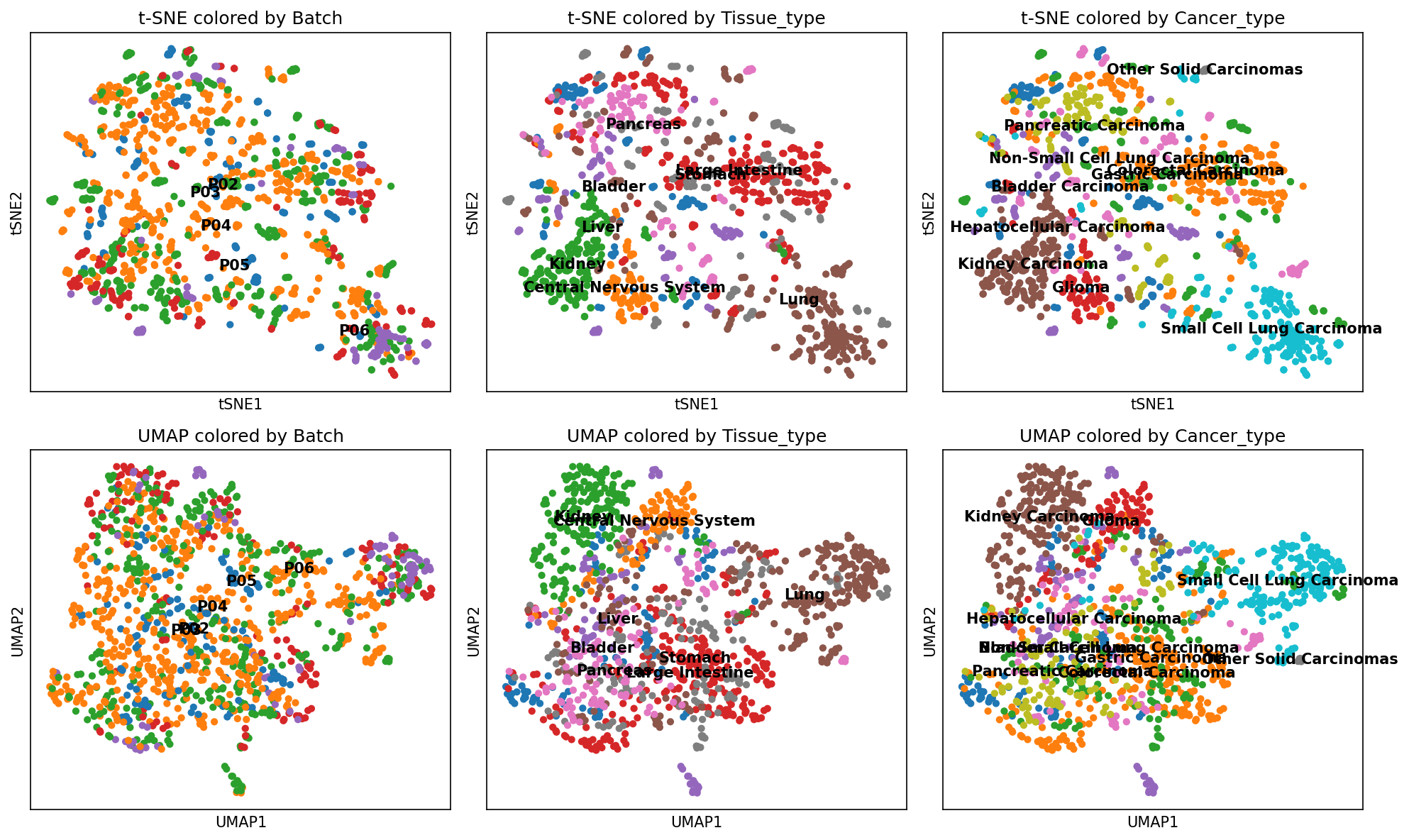
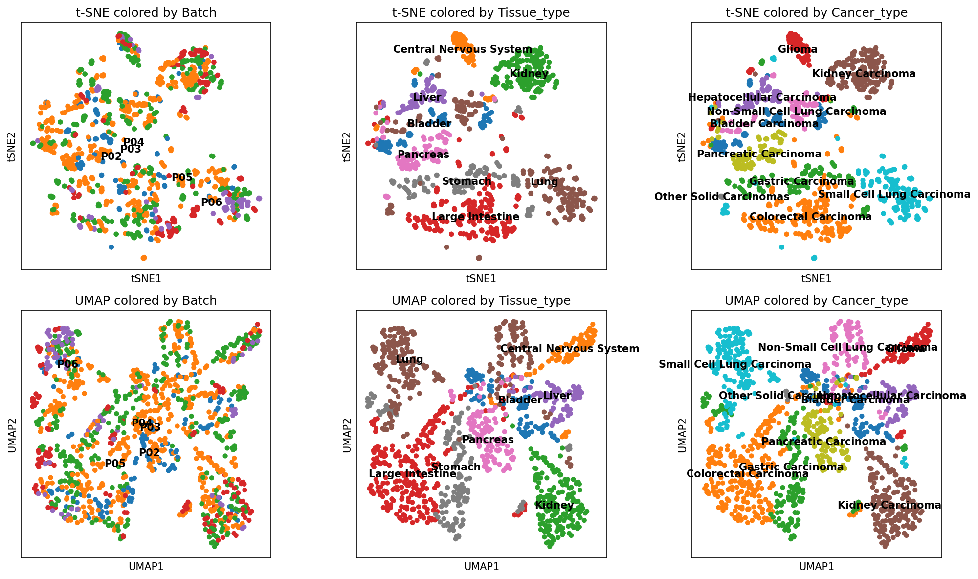
_images/PanCancer_949_celline_analysis_39_2.png

The UMAP analysis of STAVER-processed data¶

When analyzing STAVER-processed data, UMAP visualization clearly separated the 1,242 cancer cell line samples by tissue sources and cancer types (Figure RL2I and Figure RL5I). Notably, the STAVER-processed data revealed that cancer cell lines from the digestive tract, such as intestinal, gastric, and pancreatic, exhibited more molecular similarities than their nondigestive tract counterparts (lung, glioma, and kidney cancer cell lines). These findings highlighted the potential superiority of the STAVER algorithm in elucidating the intrinsic biological differences among diverse tumor cell lines.

[102]:

outpath = '~/DIA-STAVER/STAVER-nc-revised/revised-sript/figs-1/'
if not os.path.exists(outpath):
    os.makedirs(outpath)

adata_STAVER = visualize_cancer_subtypes("~/STAVER-revised/PCA/STAVER_data.csv", "~/STAVER-revised/PCA/metadata_anatation_scanpy.csv", outpath=outpath, filename = "STAVER_data_2")

WARNING: You’re trying to run this on 8202 dimensions of `.X`, if you really want this, set `use_rep='X'`.
         Falling back to preprocessing with `sc.pp.pca` and default params.

_images/PanCancer_949_celline_analysis_41_1.png

Cancer specific proteins¶

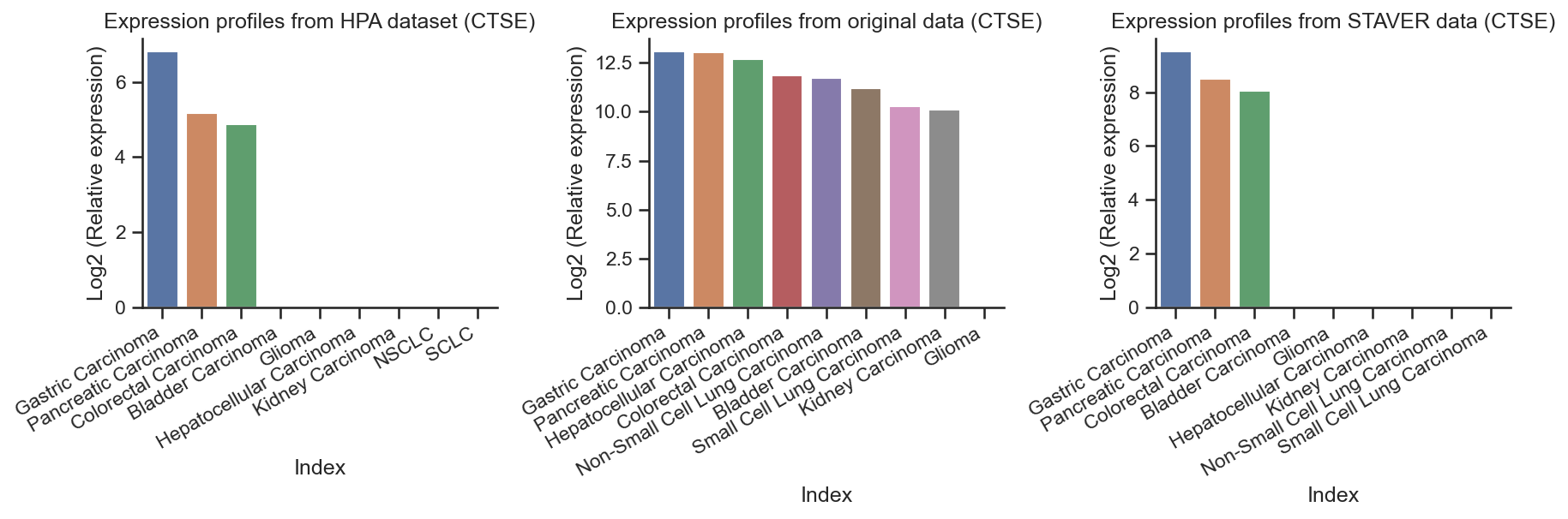
To rigorously establish the advantages of the STAVER algorithm in identifying tumor cell-specific proteins, we compared the distribution patterns of cell-specific protein expression profiles between the original and STAVER-processed data. We incorporated the Human Protein Atlas (HPA) molecular annotations of tumor cell specificity and their expression profiles across various cancer cell lines for integrated analysis.

The results demonstrated that the STAVER-processed data more accurately reflected cancer type-specific expression patterns than the original proteomic data.

[4]:

HPA_dataset = pd.read_csv("~/STAVER-nc-revised/resources/proteinatlas_56a92855.tsv", sep="\t")
HPA_dataset

[4]:

	Gene	Gene synonym	Ensembl	Gene description	Uniprot	Chromosome	Position	Protein class	Biological process	Molecular function	...	Pathology prognostics - Lung cancer	Pathology prognostics - Melanoma	Pathology prognostics - Ovarian cancer	Pathology prognostics - Pancreatic cancer	Pathology prognostics - Prostate cancer	Pathology prognostics - Renal cancer	Pathology prognostics - Stomach cancer	Pathology prognostics - Testis cancer	Pathology prognostics - Thyroid cancer	Pathology prognostics - Urothelial cancer
0	A1BG	NaN	ENSG00000121410	Alpha-1-B glycoprotein	P04217	19	58345178-58353492	Plasma proteins, Predicted intracellular prote...	NaN	NaN	...	unprognostic (1.09e-1)	unprognostic (2.59e-1)	unprognostic (2.10e-1)	unprognostic (1.47e-2)	unprognostic (1.37e-2)	unprognostic (4.19e-5)	unprognostic (2.37e-2)	unprognostic (1.94e-1)	unprognostic (1.72e-1)	unprognostic (6.72e-2)
1	A1CF	ACF, ACF64, ACF65, APOBEC1CF, ASP	ENSG00000148584	APOBEC1 complementation factor	Q9NQ94	10	50799409-50885675	Predicted intracellular proteins	mRNA processing	RNA-binding	...	unprognostic (7.38e-3)	NaN	unprognostic (1.30e-2)	unprognostic (2.46e-2)	unprognostic (1.20e-1)	unprognostic (1.90e-3)	unprognostic (1.97e-2)	unprognostic (2.77e-1)	unprognostic (2.19e-2)	unprognostic (8.50e-4)
2	A2M	CPAMD5, FWP007, S863-7	ENSG00000175899	Alpha-2-macroglobulin	P01023	12	9067664-9116229	Cancer-related genes, Candidate cardiovascular...	NaN	Protease inhibitor, Serine protease inhibitor	...	unprognostic (3.65e-2)	unprognostic (2.38e-1)	unprognostic (7.19e-2)	unprognostic (4.71e-2)	unprognostic (2.06e-2)	unprognostic (1.28e-2)	unprognostic (8.04e-3)	unprognostic (2.32e-2)	unprognostic (8.58e-2)	unprognostic (9.03e-3)
3	A2ML1	CPAMD9, FLJ25179, p170	ENSG00000166535	Alpha-2-macroglobulin like 1	A8K2U0	12	8822621-8887001	Disease related genes, Predicted intracellular...	NaN	Protease inhibitor, Serine protease inhibitor	...	unprognostic (7.58e-3)	unprognostic (2.63e-1)	unprognostic (1.57e-1)	unprognostic (1.15e-3)	unprognostic (2.03e-1)	unprognostic (1.06e-9)	unprognostic (2.28e-1)	unprognostic (3.07e-1)	unprognostic (5.88e-2)	unprognostic (2.42e-2)
4	A3GALT2	A3GALT2P, IGB3S, IGBS3S	ENSG00000184389	Alpha 1,3-galactosyltransferase 2	U3KPV4	1	33306766-33321098	Enzymes, Predicted membrane proteins	Lipid metabolism	Glycosyltransferase, Transferase	...	unprognostic (4.96e-2)	unprognostic (6.83e-2)	unprognostic (5.81e-2)	unprognostic (1.23e-1)	unprognostic (1.89e-1)	unprognostic (4.90e-8)	unprognostic (1.17e-1)	NaN	unprognostic (1.12e-2)	unprognostic (7.87e-2)
...	...	...	...	...	...	...	...	...	...	...	...	...	...	...	...	...	...	...	...	...	...
20157	ZYG11A	ZYG11	ENSG00000203995	Zyg-11 family member A, cell cycle regulator	Q6WRX3	1	52842511-52894998	Predicted intracellular proteins	Ubl conjugation pathway	NaN	...	unprognostic (2.34e-1)	unprognostic (4.56e-2)	unprognostic (2.06e-2)	unprognostic (4.01e-2)	unprognostic (1.01e-1)	unprognostic (6.15e-3)	unprognostic (2.95e-1)	unprognostic (1.21e-1)	unprognostic (3.07e-1)	unprognostic (1.02e-1)
20158	ZYG11B	FLJ13456, ZYG11	ENSG00000162378	Zyg-11 family member B, cell cycle regulator	Q9C0D3	1	52726453-52827336	Predicted intracellular proteins	Ubl conjugation pathway	NaN	...	unprognostic (1.85e-1)	unprognostic (4.84e-3)	unprognostic (5.06e-2)	unprognostic (2.76e-1)	unprognostic (6.08e-2)	prognostic favorable (9.80e-7)	unprognostic (2.22e-1)	unprognostic (3.37e-1)	unprognostic (1.13e-1)	unprognostic (9.57e-2)
20159	ZYX	NaN	ENSG00000159840	Zyxin	Q15942	7	143381295-143391111	Plasma proteins, Predicted intracellular proteins	Cell adhesion, Host-virus interaction	NaN	...	unprognostic (1.66e-3)	unprognostic (2.60e-1)	unprognostic (4.22e-1)	unprognostic (1.98e-1)	unprognostic (2.43e-1)	prognostic unfavorable (7.92e-5)	unprognostic (1.39e-1)	unprognostic (8.12e-2)	unprognostic (1.95e-1)	unprognostic (6.72e-2)
20160	ZZEF1	FLJ10821, KIAA0399, ZZZ4	ENSG00000074755	Zinc finger ZZ-type and EF-hand domain contain...	O43149	17	4004445-4143030	Predicted membrane proteins	Transcription, Transcription regulation	Activator	...	unprognostic (1.44e-2)	unprognostic (1.23e-1)	unprognostic (2.21e-2)	prognostic favorable (6.08e-4)	unprognostic (1.54e-1)	unprognostic (1.38e-3)	unprognostic (6.09e-3)	unprognostic (1.80e-1)	unprognostic (9.43e-2)	unprognostic (6.46e-2)
20161	ZZZ3	ATAC1, DKFZP564I052	ENSG00000036549	Zinc finger ZZ-type containing 3	Q8IYH5	1	77562416-77683419	Predicted intracellular proteins	Transcription, Transcription regulation	DNA-binding	...	unprognostic (2.91e-1)	unprognostic (9.67e-2)	unprognostic (1.35e-1)	unprognostic (2.83e-1)	unprognostic (1.91e-1)	unprognostic (1.71e-1)	unprognostic (3.96e-1)	unprognostic (1.95e-1)	unprognostic (3.05e-2)	unprognostic (1.43e-1)

20162 rows × 89 columns

[6]:

def get_hpa_expression_profile(protein):
    HPA = HPA_dataset[['Gene', 'RNA cell line specific nTPM']]
    HPA.set_index('Gene', inplace=True)

    return HPA.loc[protein, "RNA cell line specific nTPM"]

CTSE overexpression in Gastric, pancreatic, and colorectal cancer of HPA dataset¶

[9]:

get_hpa_expression_profile("CTSE")

[9]:

'colorectal cancer: 28.4;Esophageal cancer: 48.8;Gastric cancer: 110.7;pancreatic cancer: 35.3'

[10]:

HPA_protein_CTSE = {
    'Bladder Carcinoma': 0,
    'Colorectal Carcinoma': 28.4,
    'Gastric Carcinoma': 110.7,
    'Glioma': 0,
    'Hepatocellular Carcinoma': 0,
    'Kidney Carcinoma': 0,
    'NSCLC': 0,
    'Pancreatic Carcinoma': 35.3,
    'SCLC': 0
}


HPA_protein_CTSE = pd.DataFrame.from_dict(HPA_protein_CTSE, orient='index', columns=['CTSE'])
HPA_protein_CTSE = HPA_protein_CTSE.sort_values(by=['CTSE'], ascending=False)
HPA_protein_CTSE

[10]:

	CTSE
Gastric Carcinoma	110.7
Pancreatic Carcinoma	35.3
Colorectal Carcinoma	28.4
Bladder Carcinoma	0.0
Glioma	0.0
Hepatocellular Carcinoma	0.0
Kidney Carcinoma	0.0
NSCLC	0.0
SCLC	0.0

[11]:

STAVER = pd.read_csv("~/STAVER-revised/model-evlauate/STAVER_data.csv", index_col=0)
raw_data = pd.read_csv("~/STAVER-revised/model-evlauate/raw_data.csv", index_col=0)

[12]:

def process_data(data, target_gene):
    df = data[[target_gene, 'Cancer_type']]
    df.replace(0, np.nan, inplace=True)
    df.drop(df[df['Cancer_type'] == 'Other Solid Carcinomas'].index, inplace=True)
    df = df.groupby('Cancer_type').median()
    df = df.sort_values(by=[target_gene], ascending=False)
    return df

[13]:

rawdata_CTSE = process_data(raw_data, "CTSE")
rawdata_CTSE.sort_values(by=['CTSE'], ascending=False, inplace=True)
rawdata_CTSE

[13]:

	CTSE
Cancer_type
Gastric Carcinoma	13.064867
Pancreatic Carcinoma	13.046290
Hepatocellular Carcinoma	12.683957
Colorectal Carcinoma	11.875120
Non-Small Cell Lung Carcinoma	11.738225
Bladder Carcinoma	11.182161
Small Cell Lung Carcinoma	10.270660
Kidney Carcinoma	10.095740
Glioma	NaN

[17]:

STAVER_CTSE = process_data(STAVER, "CTSE")
STAVER_CTSE.sort_values(by=['CTSE'], ascending=False, inplace=True)
STAVER_CTSE

[17]:

	CTSE
Cancer_type
Gastric Carcinoma	9.501038
Pancreatic Carcinoma	8.500000
Colorectal Carcinoma	8.050000
Bladder Carcinoma	NaN
Glioma	NaN
Hepatocellular Carcinoma	NaN
Kidney Carcinoma	NaN
Non-Small Cell Lung Carcinoma	NaN
Small Cell Lung Carcinoma	NaN

[ ]:

mpl.rcParams['pdf.fonttype'] = 42
mpl.rcParams['figure.dpi']= 150 # 一般将dpi设置在150到300之间

custom_params = {"axes.spines.right": False, "axes.spines.top": False}
sns.set_theme(style="ticks", rc=custom_params)

def plot_barplot(df, target_col, log_transform=False, x_label=None, y_label=None, title=None, save_path=None):
    """
    Plots a barplot.

    Args:
        df (pd.DataFrame): The dataframe.
        target_col (str): The column name to be plotted as the target column.
        x_label (str): The x-axis label. Default is None.
        y_label (str): The y-axis label. Default is None.
        title (str): The title of the plot. Default is None.
        save_path (str): The path to save the image. Default is None, indicating no saving.

    Returns:
        None
    """

    plt.figure(figsize=(4, 2.7))
    if log_transform:
        sns.barplot(x=df.index, y=np.log2(df[target_col]+1))
    # Use seaborn's barplot function to plot the graph
    else:
        sns.barplot(x=df.index, y=df[target_col])

    # Set the title and axis labels
    if title:
        plt.title(title)
    if x_label:
        plt.xlabel(x_label)
    else:
        plt.xlabel("Index")
    if y_label:
        plt.ylabel(y_label)
    else:
        plt.ylabel(target_col)

    plt.xticks(rotation=30, ha='right')  # Rotate the x-axis labels for better display

    # Save the image (if save_path is specified)
    if save_path:
        plt.savefig(save_path, bbox_inches='tight')

    # Show the image
    plt.show()

[33]:

import matplotlib.pyplot as plt
import seaborn as sns
import numpy as np

# 全局的绘图参数设置
mpl.rcParams['pdf.fonttype'] = 42
mpl.rcParams['figure.dpi'] = 150

custom_params = {"axes.spines.right": False, "axes.spines.top": False}
sns.set_theme(style="ticks", rc=custom_params)

def plot_combined_barplots(datasets, target_col, titles, log_transforms, x_labels, y_labels, save_path=None):
    """
    Plots multiple barplots on a single figure, one for each dataset provided.
    """

    if not all(len(lst) == len(datasets) for lst in [titles, log_transforms, x_labels, y_labels]):
        raise ValueError("All list arguments must be of the same length as the 'datasets' list.")

    n = len(datasets)
    fig, axes = plt.subplots(1, n, figsize=(n * 4, 4.2))

    if n == 1:  # If there is only one dataset, axes will not be an array
        axes = [axes]

    for i, (df, title, log_transform, x_label, y_label) in enumerate(zip(datasets, titles, log_transforms, x_labels, y_labels)):
        ax = axes[i]
        plot_data = np.log2(df[target_col]+1) if log_transform else df[target_col]
        sns.barplot(ax=ax, x=df.index, y=plot_data)
        ax.set_title(title)
        ax.set_xlabel(x_label if x_label else "Index")
        ax.set_ylabel(y_label if y_label else target_col)

        # Set the tick parameters and label rotation
        ax.set_xticklabels(ax.get_xticklabels(), rotation=30, ha='right')

    # Adjust the left margin if needed
    plt.subplots_adjust(left=0.1)  # You might need to tweak this value

    if save_path:
        plt.savefig(save_path, bbox_inches='tight')

    plt.tight_layout()
    plt.show()


# The barplot of CTSE expression profiles
plot_combined_barplots(
    datasets=[HPA_protein_CTSE, rawdata_CTSE, STAVER_CTSE],
    target_col="CTSE",
    titles=["Expression profiles from HPA dataset (CTSE)",
            "Expression profiles from original data (CTSE)",
            "Expression profiles from STAVER data (CTSE)"],
    log_transforms=[True, False, False],
    x_labels=[None, None, None],
    y_labels=["Log2 (Relative expression)",
            "Log2 (Relative expression)",
            "Log2 (Relative expression)"],
    save_path="combined_barplots_CTSE.pdf"
)

_images/PanCancer_949_celline_analysis_53_0.png

[ ]:

# The barplot of CTSE expression profiles
plot_combined_barplots(
        datasets=[HPA_protein_CTSE, rawdata_CTSE, STAVER_CTSE],
        target_col="CTSE",
        titles=["Expression profiles from HPA dataset (CTSE)",
                "Expression profiles from original data (CTSE)",
                "Expression profiles from STAVER data (CTSE)"],
        log_transforms=[True, False, False],
        x_labels=[None, None, None],
        y_labels=["Log2 (Relative expression)",
                "Log2 (Relative expression)",
                "Log2 (Relative expression)"],
        save_path="combined_barplots_CTSE.pdf"
)

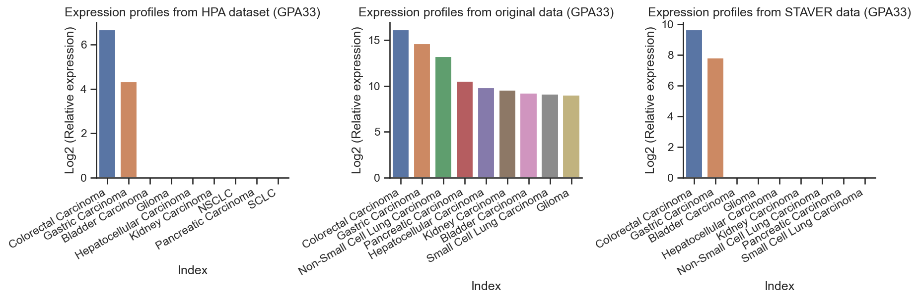
GPA33 overexpression in colorectal cancer and Gastric cancer of HPA dataset¶

[34]:

get_hpa_expression_profile("GPA33")

[34]:

'Bile duct cancer: 34.1;colorectal cancer: 100.5;Gastric cancer: 19.1'

[35]:

HPA_protein_CTSE = {
    'Bladder Carcinoma': 0,
    'Colorectal Carcinoma': 100.5,
    'Gastric Carcinoma': 19.1,
    'Glioma': 0,
    'Hepatocellular Carcinoma': 0,
    'Kidney Carcinoma': 0,
    'NSCLC': 0,
    'Pancreatic Carcinoma': 0,
    'SCLC': 0
}


HPA_protein_GPA33 = pd.DataFrame.from_dict(HPA_protein_CTSE, orient='index', columns=['GPA33'])
HPA_protein_GPA33 = HPA_protein_GPA33.sort_values(by=['GPA33'], ascending=False)
HPA_protein_GPA33

[35]:

	GPA33
Colorectal Carcinoma	100.5
Gastric Carcinoma	19.1
Bladder Carcinoma	0.0
Glioma	0.0
Hepatocellular Carcinoma	0.0
Kidney Carcinoma	0.0
NSCLC	0.0
Pancreatic Carcinoma	0.0
SCLC	0.0

[39]:

rawdata_GPA33 = process_data(raw_data, "GPA33")
rawdata_GPA33.sort_values(by=['GPA33'], ascending=False, inplace=True)
rawdata_GPA33

[39]:

	GPA33
Cancer_type
Colorectal Carcinoma	16.132530
Gastric Carcinoma	14.659133
Non-Small Cell Lung Carcinoma	13.211101
Pancreatic Carcinoma	10.548243
Hepatocellular Carcinoma	9.851693
Kidney Carcinoma	9.565263
Bladder Carcinoma	9.219547
Small Cell Lung Carcinoma	9.125549
Glioma	9.036120

[41]:

STAVER_GPA33 = process_data(STAVER, "GPA33")
STAVER_GPA33.sort_values(by=['GPA33'], ascending=False, inplace=True)
STAVER_GPA33

[41]:

	GPA33
Cancer_type
Colorectal Carcinoma	9.632096
Gastric Carcinoma	7.820000
Bladder Carcinoma	NaN
Glioma	NaN
Hepatocellular Carcinoma	NaN
Kidney Carcinoma	NaN
Non-Small Cell Lung Carcinoma	NaN
Pancreatic Carcinoma	NaN
Small Cell Lung Carcinoma	NaN

[42]:

# The barplot of GPA33 expression profiles
plot_combined_barplots(
        datasets=[HPA_protein_GPA33, rawdata_GPA33, STAVER_GPA33],
        target_col="GPA33",
        titles=["Expression profiles from HPA dataset (GPA33)",
                "Expression profiles from original data (GPA33)",
                "Expression profiles from STAVER data (GPA33)"],
        log_transforms=[True, False, False],
        x_labels=[None, None, None],
        y_labels=["Log2 (Relative expression)",
                "Log2 (Relative expression)",
                "Log2 (Relative expression)"],
        save_path="combined_barplots_GPA33.pdf"
)

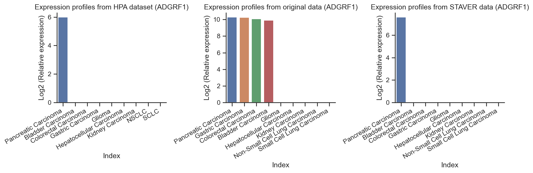
_images/PanCancer_949_celline_analysis_60_0.png

ADGRF1 overexpression in pancreatic cancer of HPA dataset¶

[43]:

get_hpa_expression_profile("ADGRF1")

[43]:

'pancreatic cancer: 62.2'

[44]:

HPA_protein_CTSE = {
    'Bladder Carcinoma': 0,
    'Colorectal Carcinoma': 0,
    'Gastric Carcinoma': 0,
    'Glioma': 0,
    'Hepatocellular Carcinoma': 0,
    'Kidney Carcinoma': 0,
    'NSCLC': 0,
    'Pancreatic Carcinoma': 62.2,
    'SCLC': 0
}


HPA_protein_ADGRF1 = pd.DataFrame.from_dict(HPA_protein_CTSE, orient='index', columns=['ADGRF1'])
HPA_protein_ADGRF1 = HPA_protein_ADGRF1.sort_values(by=['ADGRF1'], ascending=False)
HPA_protein_ADGRF1

[44]:

	ADGRF1
Pancreatic Carcinoma	62.2
Bladder Carcinoma	0.0
Colorectal Carcinoma	0.0
Gastric Carcinoma	0.0
Glioma	0.0
Hepatocellular Carcinoma	0.0
Kidney Carcinoma	0.0
NSCLC	0.0
SCLC	0.0

[45]:

rawdata_ADGRF1 = process_data(raw_data, "ADGRF1")
rawdata_ADGRF1.sort_values(by=['ADGRF1'], ascending=False, inplace=True)
rawdata_ADGRF1

[45]:

	ADGRF1
Cancer_type
Pancreatic Carcinoma	10.272240
Gastric Carcinoma	10.256628
Colorectal Carcinoma	10.093484
Bladder Carcinoma	9.910033
Glioma	NaN
Hepatocellular Carcinoma	NaN
Kidney Carcinoma	NaN
Non-Small Cell Lung Carcinoma	NaN
Small Cell Lung Carcinoma	NaN

[46]:

STAVER_ADGRF1 = process_data(STAVER, "ADGRF1")
STAVER_ADGRF1.sort_values(by=['ADGRF1'], ascending=False, inplace=True)
STAVER_ADGRF1

[46]:

	ADGRF1
Cancer_type
Pancreatic Carcinoma	7.594326
Bladder Carcinoma	NaN
Colorectal Carcinoma	NaN
Gastric Carcinoma	NaN
Glioma	NaN
Hepatocellular Carcinoma	NaN
Kidney Carcinoma	NaN
Non-Small Cell Lung Carcinoma	NaN
Small Cell Lung Carcinoma	NaN

[47]:

# The barplot of ADGRF1 expression profiles
plot_combined_barplots(
        datasets=[HPA_protein_ADGRF1, rawdata_ADGRF1, STAVER_ADGRF1],
        target_col="ADGRF1",
        titles=["Expression profiles from HPA dataset (ADGRF1)",
                "Expression profiles from original data (ADGRF1)",
                "Expression profiles from STAVER data (ADGRF1)"],
        log_transforms=[True, False, False],
        x_labels=[None, None, None],
        y_labels=["Log2 (Relative expression)",
                "Log2 (Relative expression)",
                "Log2 (Relative expression)"],
        save_path="combined_barplots_ADGRF1.pdf"
)

_images/PanCancer_949_celline_analysis_66_0.png

The reproducibility of the STAVER algorithm in identifying the previously reported tumor biomarkers¶

To further validate the superior reproducibility of the STAVER algorithm in identifying tumor biomarkers, a systematic literature review was conducted. According to the systematic literature review, a series of cancer biomarkers were selected to further evaluate the STAVER algorithm (Table RL1 and Table RL4). We utilized the original and STAVER-processed proteomic data to examine the expression differences of these previously reported cancer biomarkers across diverse cancer cell lines.

The results demonstrated that the STAVER algorithm more accurately identify the previously reported tumor biomarkers with high reproducibility.

[49]:

reported_biomrkers = pd.read_clipboard()
reported_biomrkers

[49]:

	Tissue Type	Cancer Type	Reported Biomarker	Reference	PMID
0	Liver	Hepatocellular carcinoma	DCP	Journal of Hepatology, 2023	PMID: 37683735
1	Liver	Hepatocellular carcinoma	HSP70	Journal of hepatology, 2009	PMID: 19231003
2	Liver	Hepatocellular carcinoma	GGT1	Gastroenterology, 2017; BMC Cancer, 2019	PMID: 28711626; PMID: 31455253
3	Liver	Hepatocellular carcinoma	A1CF	Cell reports, 2019; The JCI, 2021	PMID: 31597092; PMID: 33445170
4	Kidney	Kidney cancer	CA9	European urology, 2014; Cancer research, 1997	PMID: 24821582; PMID: 9230182
5	Kidney	Kidney cancer	CD70	Cancer research, 2006	PMID: 16489038
6	Gastric	Gastric cancer	ERRB2	Annals of oncology, 2008	PMID: 18441328
7	Gastric	Gastric cancer	AGR3	In vivo, 2023	PMID: 36593009
8	Colorectal	Colorectal cancer	MUC2	Gastroenterology, 2005;	PMID: 16285957
9	Colorectal	Colorectal cancer	EPCAM	British journal of cancer, 2014	PMID: 24786601
10	Colorectal	Colorectal cancer	CDX2	Annals of oncology, 2017	PMID: 28328000
11	Colorectal	Colorectal cancer	MUC13	Oncogene, 2019	PMID: 31427737
12	Brain	Glioma	GFAP	Brain, 2007; Biosens Bioelectron, 2020	PMID: 17998256; PMID: 33160234
13	Brain	Glioma	NES	Cancer cell, 2020; Mol Neurobiol, 2017	PMID: 32396858; PMID: 26768429
14	Pancreas	Pancreatic cancer	MUC1	Journal of gastroenterology,2003	PMID: 14714254
15	Pancreas	Pancreatic cancer	ANO1	PNAS, 2019	PMID: 31182586
16	Lung	Non-small cell lung cancer	KRT5	Cancer cell, 2022	PMID: 36368318
17	Lung	Non-small cell lung cancer	DSC3	Journal of thoracic oncology, 2011	PMID: 21623236
18	Lung	Small cell lung cancer	CHGA	Cell reports, 2020	PMID: 33086069
19	Lung	Small cell lung cancer	NCAM1	Cancer cell, 2022	PMID: 36368318

Reported_cancer_biomarkers

All the results are shown in the above figure and can be reproduced with the R script boxplot_949_PanCancer.R.

The robustness and broad applicability of the STAVER algorithm for disease diagnosis and classification.¶

To validate the outstanding advantages of the STAVER algorithm for potential clinical decision-making, we comprehensively evaluated the generalization performance and prediction accuracy of classification models constructed based on the above tumor biomarkers.

To illustrate the robustness and broad applicability of the STAVER algorithm, we constructed three separate benchmark classification models based on different algorithms, including decision tree-based random forest, gradient boosting-based XGBoost, and linear regression-based logistic regression models (Materials and methods section).

As a result, compared to the original proteomic data, the classification models constructed based on STAVER-processed data exhibited increased generalization performance in distinguishing specific cancer-type cell lines.

See the PanCancer_949_cellline_models.ipynb for more details.

[ ]: